
TensorFlow 2 tutorial: Writing and testing TensorFlow 2 Linear Regression Example
In this section we will show you how you can write your own Linear Regression model in TensorFlow 2. You will learn to develop your own model, generate data, train and validate Linear Regression Model in TensorFlow 2.
TensorFlow is very popular machine learning and mathematical computing library which can be used to develop various kind of deep learning models. In this section we will see the steps to develop a simple Linear Regression model. You can run this program in your local computer or use the the Google Colab for running this application. This tutorial is for beginners learning the machine learning application development in TensorFlow. You can check many TensorFlow 2.x tutorials by visiting our TensorFlow 2.x tutorial section.
Linear Regression is supervised machine learning algorithm which is one of the most used machine learning algorithm. This algorithm is easy and most popular supervised machine learning algorithm used in Data Science.
Writing Linear Regression model in TensorFlow 2
First all install TensorFlow 2.x on your computer as we will use TensorFlow 2 for developing the program. You can check our tutorial Install TensorFlow 2.3.0 on Google Colab if TensorFlow is not installed on your computer. Here are the libraries you should import in your program:
#Import required Libraries
import tensorflow as tf
import numpy as np
import matplotlib.pyplot as plt
We are importing TensorFlow, numpy and matplotlib library with the help of above code.
Here is complete video tutorial of creating your first Linear Regression Model in TensorFlow 2.0:
Now we will define our Linear Regression model with the help of following code:
# Define a Linear model
class LinearModel(object):
    def __init__(self):
        self.W = tf.Variable(12.0)
        self.b = tf.Variable(-6.1)

    def __call__(self, inputs):
        return self.W * inputs + self.b
Now we will define the cost funtion for our model. Here is the code of cost function:
#Define Loss Function
def compute_loss(y_true, y_pred):
    return tf.reduce_mean(tf.square(y_true-y_pred))
Now the next step is to initialize the model:
#Instantiate Linear Regression Model
model = LinearModel()
Now we will define the weight and bias with the help of following code:
# Define the weight and bias
weight = 2.5
bias = 1.0
The next step is to generate or load the data for training the model. If you are working on the commercial project then you will have to write program for pre-processing of data. In this example we are generating data with following code:
# Generate Data
data = 100
inputs  = tf.random.normal(shape=[data])
noise   = tf.random.normal(shape=[data])
outputs = inputs * weight + bias + noise
You can check the generated data by printing with the help of following code:
print(inputs)
print(noise)
print(outputs)
Define the data visualization function to be used to display graph during training.
# Model visualization function to generate graph during training
def plot(epoch):
    plt.scatter(inputs, outputs, c='b')
    #plt.scatter(inputs, model(inputs), c='m')
    plt.plot(inputs, model(inputs),  c='r', label ='Fitted line')
    plt.title("epoch %2d, loss = %s" %(epoch, str(compute_loss(outputs, model(inputs)).numpy())))
    plt.legend()
    plt.draw()
    plt.ion()
    plt.pause(1)
    plt.close()
Now you can run the model training with the help of following code:
Ws, bs = [], []
epochs = range(30)
# Define a training loop
learning_rate = 0.1
for epoch in epochs:
with tf.GradientTape() as tape:
loss = compute_loss(outputs, model(inputs))
dW, db = tape.gradient(loss, [model.W, model.b])
Ws.append(model.W.numpy())
bs.append(model.b.numpy())
model.W.assign_sub(learning_rate * dW)
model.b.assign_sub(learning_rate * db)
print("=> epoch %2d: w_true= %.2f, w_pred= %.2f; b_true= %.2f, b_pred= %.2f, loss= %.2f" %(
epoch+1, weight, model.W.numpy(), bias, model.b.numpy(), loss.numpy()))
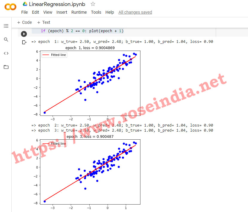
if (epoch) % 2 == 0: plot(epoch + 1)
Here is the output of the model training:
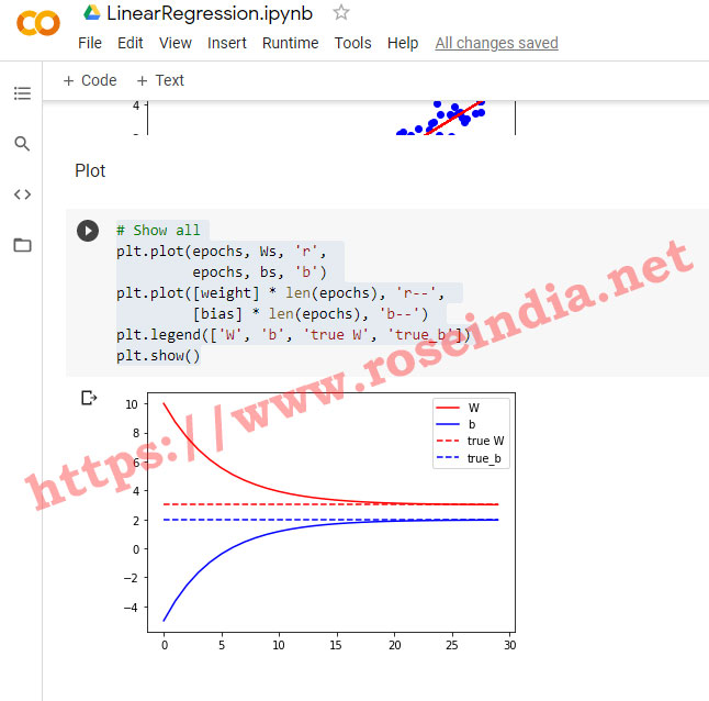
Following code will show the model training progress in the graphical view:
# Show all
plt.plot(epochs, Ws, 'r',
         epochs, bs, 'b')
plt.plot([weight] * len(epochs), 'r--',
         [bias] * len(epochs), 'b--')
plt.legend(['W', 'b', 'true W', 'true_b'])
plt.show()
Here is the output image:
Here is the complete code of the Linear Regression model we developed in TensorFlow 2.0:
import tensorflow as tf
import numpy as np
import matplotlib.pyplot as plt

"""Now we will define model and loss function"""

# Define a Linear model
class LinearModel(object):
    def __init__(self):
        self.W = tf.Variable(12.0)
        self.b = tf.Variable(-6.1)

    def __call__(self, inputs):
        return self.W * inputs + self.b

#Define Loss Function
def compute_loss(y_true, y_pred):
    return tf.reduce_mean(tf.square(y_true-y_pred))

"""Initialize our linear regression model.

"""

#Instantiate Linear Regression Model
model = LinearModel()

"""Define weight and bias for the model"""

# Define the weight and bias
weight = 2.5
bias = 1.0

"""Prepare Training Data"""

# Generate Data
data = 100
inputs  = tf.random.normal(shape=[data])
noise   = tf.random.normal(shape=[data])
outputs = inputs * weight + bias + noise

"""Check Generated data:

"""

print(inputs)

"""Print noise data:

"""

print(noise)

"""Print outputs:"""

print(outputs)

"""Define the data visualizatin function to be used to display graph during training."""

# Model visualization function to generate graph during training
def plot(epoch):
    plt.scatter(inputs, outputs, c='b')
    #plt.scatter(inputs, model(inputs), c='m')
    plt.plot(inputs, model(inputs),  c='r', label ='Fitted line')
    plt.title("epoch %2d, loss = %s" %(epoch, str(compute_loss(outputs, model(inputs)).numpy())))
    plt.legend()
    plt.draw()
    plt.ion()
    plt.pause(1)
    plt.close()

"""Training Loop"""

Ws, bs = [], []

epochs = range(30)

# Define a training loop
learning_rate = 0.1
for epoch in epochs:
    with tf.GradientTape() as tape:
        loss = compute_loss(outputs, model(inputs))

    dW, db = tape.gradient(loss, [model.W, model.b])

    Ws.append(model.W.numpy())
    bs.append(model.b.numpy())

    model.W.assign_sub(learning_rate * dW)
    model.b.assign_sub(learning_rate * db)

    print("=> epoch %2d: w_true= %.2f, w_pred= %.2f; b_true= %.2f, b_pred= %.2f, loss= %.2f" %(
          epoch+1, weight, model.W.numpy(), bias, model.b.numpy(), loss.numpy()))
    if (epoch) % 2 == 0: plot(epoch + 1)

"""Plot"""

# Show all
plt.plot(epochs, Ws, 'r',
         epochs, bs, 'b')
plt.plot([weight] * len(epochs), 'r--',
         [bias] * len(epochs), 'b--')
plt.legend(['W', 'b', 'true W', 'true_b'])
plt.show()
You can download the example from:
Related TensorFlow 2 Tutorials